Research update: Towards a Law of Iterated Expectations for Heuristic Estimators
Last week, ARC released a paper called Towards a Law of Iterated Expectations for Heuristic Estimators, which follows up on previous work on formalizing the presumption of independence. Most of the work described here was done in 2023.
A brief table of contents for this post:
- What is a heuristic estimator? (One example and three analogies.)
- How might heuristic estimators help with understanding neural networks? (Three potential applications.)
- Formalizing the principle of unpredictable errors for heuristic estimation (the technical meat of the paper).
In "Formalizing the Presumption of Independence", we defined a heuristic estimator to be a hypothetical algorithm that estimates the values of mathematical expression based on arguments. That is, a heuristic estimator is an algorithm \(\mathbb{G}\) that takes as input
- A formally specified real-valued expression \(Y\); and
- A set of formal "arguments" \(\pi_1, \ldots, \pi_m\) –
– and outputs an estimate of the value of \(Y\) that incorporates the information provided by \(\pi_1, \ldots, \pi_m\). We denote this estimate by \(\mathbb{G}(Y \mid \pi_1, \ldots, \pi_m)\).[1]
In that paper, we introduced the following question: is there a computationally efficient heuristic estimator that formalizes intuitively valid reasoning about the values of mathematical quantities based on arguments? We studied the question by introducing intuitively desirable coherence properties (one such property is linearity: a heuristic estimator's estimate of \(X+Y\) should equal its estimate of \(X\) plus its estimate of \(Y\)) and working to satisfy those properties. Ultimately, we left the question open.
The main technical contribution of our new work is to outline a new type of coherence property: a heuristic estimator should not be able to predict its own errors. We call this intuitive statement the principle of unpredictable errors. The principle is loosely inspired by the law of iterated expectations from probability theory, as well as the martingale property: a Bayesian reasoner's estimate of their future estimate of a quantity should be equal to its current estimate. One of the main purposes of this work is to explore ways to formalize this principle.
Our paper is structured as follows:
- We begin by explaining the core motivating intuition behind heuristic estimators through three analogies: proof verification, conditional expectations, and subjective probabilities.
- We explain why we believe in the principle of unpredictable errors. We then describe a natural attempt to formalize the principle: to simplify, we ask that \(\mathbb{G}(Y - \mathbb{G}(Y \mid \Pi) \mid \Pi) = 0\) for every \(\)expression \(Y\) and set of arguments \(\Pi = {\pi_1, \ldots, \pi_m}\). (We call this property iterated estimation and also define a more complex property which we call error orthogonality.) We then discuss important drawbacks of this formalization, which stem from the nested \(\mathbb{G}\)'s in the definition of the properties.
- Taking inspiration from these properties, we define a cluster of accuracy properties, which – roughly speaking – replace the outer \(\mathbb{G}\) with an expected value over a distribution of expressions \(Y\). The simplest of these properties states that \(\)\(\mathbb{E}_{Y \sim \mathcal{D}}[Y - \mathbb{G}(Y \mid \Pi) \mid \Pi] = 0\).
- We examine the accuracy properties in the context of two estimation problems: (1) estimating the expected product of jointly normal random variables and (2) estimating the permanent of a matrix. In both cases, we encounter barriers to satisfying the accuracy properties, even when the set of heuristic arguments is small and simple. This leads us to reject accuracy as a formalization of the principle of unpredictable errors. We leave open the question of how to correctly formalize this principle.
- We conclude with a discussion of our motivations for pursuing this line of research. While the problem of heuristic estimation is deeply interesting from a theoretical standpoint, we believe that it could have applications for understanding the behavior of neural networks. We discuss three potential applications of heuristic estimation to understanding neural network behavior: mechanistic anomaly detection,[2] safe distillation, and low probability estimation.
This blog post summarizes the paper, with proportionally more emphasis on the main ideas and less emphasis on the mathematical details.
What is a heuristic estimator?
In "Formalizing the Presumption of Independence", we described a heuristic estimator as an efficient program that forms a "subjective expected value" of a quantity based on arguments. We gave several examples of heuristic estimation, such as estimating the number of twin primes in a given range and estimating the probability that some 256-bit input to the SHA-256 circuit has an all-zeros output.
In our new paper, we expand on the intuition behind heuristic estimators through one example and three analogies.
Example: Sum of sixth digits of square roots
Let \(d_6(\sqrt{n})\) denote the sixth digit of \(\sqrt{n}\) past the decimal point (in base 10), and let \(Y := \sum_{n = 101}^{120} d_6(\sqrt{n})\). What is your best guess for the value of \(Y\)?
Without actually calculating any square roots, your best bet is to estimate each of the twenty digits as \(4.5\) (the average of 0 through 9); this gives an estimate of \(20 \cdot 4.5 = 90\). This is perhaps how we want our heuristic estimator to behave when given no arguments; in other words, we want our heuristic estimator \(\mathbb{G}\) to satisfy \(\mathbb{G}(Y \mid \emptyset) = 90\).[3]
Now, let \(\pi_n\) be a computation of the sixth digit of \(\sqrt{n}\). When given \(\pi_n\) as an argument, \(\mathbb{G}\) should update its estimate of \(Y\) accordingly. For example, the sixth digit of \(\sqrt{101}\) happens to be 5. Correspondingly, we would like \(\mathbb{G}(Y \mid \pi_{101}) = 5 + 19 \cdot 4.5 = 90.5\). If \(\mathbb{G}\) is additionally given \(\pi_{102}\), which shows that the sixth digit of \(\sqrt{102}\) is 4, \(\mathbb{G}\) should again update its estimate: \(\mathbb{G}(Y \mid \pi_{101}, \pi_{102}) = 5 + 4 + 18 \cdot 4.5 = 90\) – and so on. If \(\mathbb{G}\) is given all of \(\pi_{101}\) through \(\pi_{120}\), then it should be able to compute the correct answer.
(The purpose of this example is to provide a very simple and intuitive picture of how we expect \(\mathbb{G}\) to update based on arguments. In practice, we expect the arguments given to \(\mathbb{G}\) to be much more complex.)
Analogy #1: Proof verification
A proof verifier is a program that takes as input a formal mathematical statement and a purported proof of the statement, and checks whether the proof is valid. This is very similar to a heuristic estimator, which is a program that takes as input a formal mathematical expression and some arguments about the expression, and outputs an estimate of the value of the expression in light of those arguments.
Just as a proof verifier does not attempt to generate its own proof of the statement – it just checks whether the given proof is valid – a heuristic estimator does not attempt to estimate the given quantity using its own arguments. Its only purpose is to incorporate the arguments that it is given into an estimate. Moreover, we can think of a heuristic estimator as a generalized proof verifier: we expect heuristic estimators to respect proofs, in the sense that if an argument \(\pi\) proves that \(\ell \le Y \le h\), then \(\mathbb{G}(Y \mid \pi)\) should lie between \(\ell\) and \(h\). (See Section 4 here.)
This table (adapted from chapter 9 here) illustrates the analogy between proof verifiers and heuristic estimators in more detail.
| Heuristic estimation | Proof verification |
| Heuristic estimator | Proof verifier |
| Formal mathematical expression | Formal mathematical statement |
| List of heuristic arguments | Purported proof of statement |
| Formal language for heuristic arguments | Formal language for proofs |
| Desiderata for estimator | Soundness and completeness |
| Algorithm's estimate of expression | Verifier's output (accept or reject) |
Analogy #2: Conditional expectation
In some ways, a heuristic estimator is analogous to a conditional expected value. For a random variable \(X\) and event \(A\), \(\mathbb{E}[X \mid A]\) is the average value of \(X\) conditioned on \(A\) – or put otherwise, it is the estimate of \(X\) given by an observer who knows that \(A\) occurred and nothing else. Similarly, \(\mathbb{G}(Y \mid \Pi)\) is the estimate of \(Y\) given by an observer who has not computed the exact value of \(Y\) and has instead only done the computations described in the arguments in \(\Pi\). Although there is a particular correct value of \(Y\), the observer does not know this value, and \(\mathbb{G}(Y \mid \Pi)\) is a subjective "best guess" about \(Y\) given only \(\Pi\). Both quantities can thus be thought of as a best guess conditional on a state of knowledge.
Analogy #3: Subjective probabilities and estimates
Perhaps the best intuitive explanation of heuristic estimation is this: a heuristic estimator is a procedure that extracts a subjective expectation from a state of knowledge. Under this view, \(\Pi\) formally describes a set of facts known by an observer, and \(\mathbb{G}(Y \mid \Pi)\) is a subjective estimate of \(Y\) in light of those facts.
By "subjective expectation", we mean "expected value under the subjectivist view of probability". The subjectivist view of probability interprets probability as the subjective credence of an observer. For example, suppose that I have chosen a random number \(p\) uniformly from \([0, 1]\), minted a coin that comes up heads with probability \(p\), and then flipped it. What is the probability that the coin came up heads?
To an observer who only knows my procedure (but doesn't know \(p\)), the subjective probability that the coin came up heads is \(\frac{1}{2}\). To an observer who knows \(p\) (but hasn't seen the outcome of the coin flip), the subjective probability that the coin came up heads is \(p\). And to an observer who saw the outcome of the coin flip, the probability is either 0 (if the coin came up tails) or 1 (if it came up heads).
Much as observers can have subjective probabilities, they can also have subjective expectations. For example, a typical mathematician does not know the 6th digit past the decimal point of \(\sqrt{101}\), but would subjectively assign a uniform probability to each of \(0, \ldots, 9\), which means that their subjective expectation for the digit is \(4.5\). Recalling our example from earlier, the mathematician's subjective expectation for \(Y := d_6(\sqrt{101}) + \ldots + d_6(\sqrt{120})\) is \(20 \cdot 4.5 = 90\). But if the mathematician were to learn that \(d_6(\sqrt{101}) = 5\), they would update their subjective expectation to \(90.5\). This is exactly how we want our heuristic estimator \(\mathbb{G}\) to operate.
How can heuristic estimation help us understand neural networks?
While heuristic estimation is a deep and interesting topic in its own right, our research is primarily motivated by potential applications to understanding neural network behavior.
Historically, researchers mostly understood neural network behavior through empirical observation: the model's input-output behavior on particular inputs. However, this approach has important drawbacks: for example, any understanding gained about a model's behavior on one input distribution may not carry over to a different input distribution.
More recently, there has been substantial work on neural network interpretability via understanding how models internally represent concepts. Interpretability research aims to address the barriers faced by methods that rely only on input-output behavior. However, current interpretability techniques tend to only work under strong assumptions about how neural networks represent information (such as the linear representation hypothesis). Also, for the most part, these techniques can only work insofar as neural representations of concepts are understandable to humans.
A different approach is formal verification: formally proving properties of neural networks such as accuracy or adversarial robustness. While formal verification does not rely on human understanding, we believe that formally proving tight bounds about interesting behaviors of large neural networks is out of reach.
By contrast, heuristic arguments about properties of neural networks may have important advantages of both formal verification and interpretability. On the one hand, heuristic arguments (like proofs) are formal objects that are not required to be human-understandable. This means that heuristic arguments could be used to reason about properties of neural networks for which no compact human-understandable explanation exists. On the other hand, heuristic arguments (like interpretability approaches) do not require perfect certainty to be considered valid. This allows for short heuristic arguments of complex properties of large models, even when no short proofs of those properties exist.[4] (See our earlier post on surprise accounting for further discussion.)
In the rest of this section, I will give three examples of problems that we believe cannot be solved in full generality with current approaches, but that they may be solvable with heuristic arguments. (All three examples will just be sketches of possible approaches, with many details left to be filled in.)
Mechanistic anomaly detection
Let \(M\) be a neural network that was trained on a distribution \(\mathcal{D}\) of inputs \(x\) using the loss function \(L(x, M(x))\).[5] Suppose that \(M\) successfully learns to achieve low loss: that is, \(\mathbb{E}_{x \sim \mathcal{D}}[L(x, M(x))]\) is small. Let \(x^\ast\) be a (perhaps out-of-distribution) input. We call \(x^\ast\) a mechanistic anomaly for \(M\) if \(M\) gets a low loss on \(x^\ast\), but for a "different reason" than the reason why it gets low average loss on \(\mathcal{D}\). In other words, mechanistic anomalies are inputs on which \(M\) acts in a seemingly reasonable way, but via anomalous internal mechanisms.[6] To detect a mechanistic anomaly, reasoning about \(M\)'s internal structure may be necessary.
How could we use a heuristic estimator to detect mechanistic anomalies? Suppose that we find a set of arguments \(\Pi\) such that the following quantity is low:[7]
\[\mathbb{G}(\mathbb{E}_{x \sim \mathcal{D}}[L(x, M(x))] \mid \Pi).\]
That is, \(\Pi\) explains why \(M\) attains low average loss on \(\mathcal{D}\).[8] Given an out-of-distribution input \(x^\ast\) such that \(L(x^\ast, M(x^\ast))\) is once again low, we consider the quantity \(\mathbb{G}(L(x^\ast, M(x^\ast)) \mid \Pi)\). This represents a heuristic estimate of \(M\)'s loss on \(x^\ast\) based only on the reasons provided in \(\Pi\): that is, based only on the facts necessary to explain \(M\)'s low loss on \(\mathcal{D}\).
If \(\mathbb{G}(L(x^\ast, M(x^\ast)) \mid \Pi)\) is (correctly) low, then the reasons why \(M\) performs well on \(\mathcal{D}\) also explain why \(M\) performs well on \(x^\ast\). By contrast, if \(\mathbb{G}(L(x^\ast, M(x^\ast)) \mid \Pi)\) is (incorrectly) high, then \(M\) performs well on \(x^\ast\) for a different reason that why \(M\) performs well on \(\mathcal{D}\). As a result, we flag \(x^\ast\) as a mechanistic anomaly for \(M\).
(See here for a more detailed discussion of mechanistic anomaly detection.)
Safe distillation
Let \(f\) ("fast") and \(s\) ("slow") be two neural networks that were trained on a distribution \(\mathcal{D}\) of inputs to complete the same task. Thus, \(f\) and \(s\) behave similarly on \(\mathcal{D}\). Suppose that we trust \(s\) to be aligned (e.g. we trust \(s\) to generalize well off-distribution) and do not similarly trust \(f\), but that \(s\) is much slower than \(f\).[9] Given an out-of-distribution input \(x^\ast\), we would like to estimate \(s(x^\ast)\) without running \(s\). We could do this by running \(f\) on \(x^\ast\) and hoping that \(f\) generalizes well to \(x^\ast\). However, this approach is not very robust. Instead, we can attempt to use the internal activations of \(f\) to predict \(s(x^\ast)\).
Concretely, suppose for simplicity that \(f\) and \(s\) output vectors, and suppose that we find a set of arguments \(\Pi\) such that the following quantity is low:
\[\mathbb{G}(\mathbb{E}_{x \sim \mathcal{D}}[\lVert{f(x) - s(x)\rVert^2] \mid \Pi).}\]
That is, \(\Pi\) explains why \(f\) and \(s\) produce similar outputs on \(\mathcal{D}\). Given an out-of-distribution input \(x^\ast\), we consider the quantity
\[\mathbb{G}(s(x^\ast) \mid \Pi, \text{computational trace of }f\text{ on }x^\ast).\]
This represents a heuristic estimate of \(s(x^\ast)\) given the computations done by \(f\) and the argument \(\Pi\) for why \(f\) and \(s\) are similar on \(\mathcal{D}\). If the reason why \(f\) and \(s\) behave similarly on \(\mathcal{D}\) also extends to \(x^\ast\), then \(\mathbb{G}\) will correctly estimate \(s(x^\ast)\) to be similar to \(f(x^\ast)\). On the other hand, if the reason why \(f\) and \(s\) behave similarly on \(\mathcal{D}\) does not extend to \(x^\ast\), then \(\mathbb{G}\)'s estimate of \(s(x^\ast)\) may be different from \(f(x^\ast)\). This estimate may be more robust to distributional shifts, because it is based on mechanistic reasoning about how \(f\) and \(s\) work.
Safe distillation and mechanistic anomaly detection are closely related problems. The key difference is that in the safe distillation problem, we have a trusted model \(s\). This makes the setting easier; in exchange, we can hope to do more Concretely, we expect \(f\) and \(s\) to differ on \(x^\ast\) if \(x^\ast\) is a mechanistic anomaly for \(f\) (but not for \(s\)). Solving the safe distillation problem would allow us to not only detect \(x^\ast\) as an anomalous input, but to predict \(s(x^\ast)\) from the internals of \(f\). An algorithm for predicting \(s(x^\ast)\) from \(f\)'s internals would act as a distillation of \(s\), but – unlike \(f\) – it would be a safe distillation (hence the name).
Low probability estimation
Let \(M\) be a neural network that was trained on a distribution \(\mathcal{D}\). Let \(C\) (for "catastrophe") be a different neural network that checks the output of \(M\) for some rare but highly undesirable behavior: \(C(M(x))\) returns \(1\) if \(M\) exhibits the undesirable behavior on \(x\), and \(0\) otherwise. We may wish to estimate \(\mathbb{E} _ {x \sim \mathcal{D}}[C(M(x)) = 1]\), and we cannot do so by sampling random inputs \(x \sim \mathcal{D}\) because \(C\) outputs \(1\) very rarely. Suppose that we find a set of arguments \(\Pi\) that explains the mechanistic behavior of \(M\) and \(C\). If this explanation is good enough, then \(\mathbb{G}(\mathbb{E} _ {x \sim \mathcal{D}}[C(M(x))] \mid \Pi)\) will be a high-quality estimate of this probability. Additionally, we may use \(\mathbb{G}\) to more efficiently check \(M\)'s behavior on particular inputs: given an input \(x^\ast\), the quantity
\[\mathbb{G}(C(M(x^\ast)) \mid \Pi, \text{computational trace of }M\text{ on }x^\ast)\]
represents an estimate of the likelihood that \(C(M(x^\ast)) = 1\) based on the computations done by \(M\). This is especially useful if \(C\) is slow and running it on every output of \(M\) is prohibitively expensive.
A few weeks ago, we published a blog post on this potential application. In the blog post, we discussed layer-by-layer activation modeling as a possible approach to the problem. We believe that solving the problem in full generality would require sophisticated activation models that can represent a rich space of possible distributional properties of neural activations. This is similar to our goal of developing a conception of heuristic arguments that is rich enough to point out essentially any structural property of a neural network. Activation modeling and heuristic estimation are different perspectives on the same underlying approach.
With this motivation for heuristic estimators in mind, let us now discuss what properties they ought to satisfy.
Formalizing the principle of unpredictable errors
Recall from Analogy #3 that we should expect heuristic estimators to behave a lot like Bayesian reasoners. In fact, perhaps heuristic estimators should satisfy formal properties that Bayesian reasoners satisfy.
One property of Bayesian reasoning is known as the martingale property, which states that a Bayesian reasoner's estimate (i.e. subjective expectation) of their future estimate of some quantity should equal their current estimate of the quantity. Or more informally, a Bayesian reasoner cannot predict the direction in which they will update their estimate in light of new information. If they could, then they would make that update before receiving the information.
By analogy, a heuristic estimator ought not to be able to predict the direction of its own errors. We call this the principle of unpredictable errors. While this principle is informal, formalizing it could be a first step toward searching for an intuitively reasonable heuristic estimator. This motivates trying to find a satisfying formalization of the principle. Below, we will discuss two approaches for formalization: a subjective approach and an objective approach.
The subjective approach: Iterated estimation and error orthogonality
Our subjective approach to formalizing the principle of unpredictable errors involves two properties that we call iterated estimation and error orthogonality.
We say that \(\mathbb{G}\) satisfies the iterated estimation property if for all expressions \(Y\) and for all sets of arguments \(\Pi\) and \(\Pi' \subseteq \Pi\), we have
\[\mathbb{G}(\mathbb{G}(Y \mid \Pi) \mid \Pi') = \mathbb{G}(Y \mid \Pi').\]
The sense in which the iterated estimation property formalizes the principle of unpredictable errors is fairly straightforward. The expression \(\mathbb{G}(Y \mid \Pi')\) represents the heuristic estimator's belief given only the arguments in \(\Pi'\). The expression \(\mathbb{G}(Y \mid \Pi)\) represents the estimator's belief given a larger set of arguments. The iterated estimation property states that the estimator's belief (given \(\Pi'\)) about what their belief about \(Y\) would be if presented with all of \(\Pi\) is equal to their current belief about \(Y\). This closely mirrors the martingale property of Bayesian reasoners. It is also directly analogous to the law of iterated expectations from probability theory, hence the name "iterated estimation."[10]
As an example, let \(Y, \pi_{101}, \pi_{102}\) be defined as in our earlier example with the square roots. Let \(\Pi = {\pi_{101}, \pi_{102}}\) and \(\Pi' = {\pi_{101}}\). As discussed above, we have \(\mathbb{G}(Y \mid \pi_{101}) = 90.5\) (because the sixth digit of \(\sqrt{101}\) is \(5\)). The iterated estimation property states that \(\mathbb{G}(\mathbb{G}(Y \mid \pi_{101}, \pi_{102}) \mid \pi_{101})\) is also equal to \(90.5\). In other words, after \(\mathbb{G}\) has learned \(\pi_{101}\) (but not yet \(\pi_{102}\)), its estimate of what its belief of \(Y\) will be after learning \(\pi_{102}\) is its current estimate of \(Y\), namely \(90.5\).
We say that \(\mathbb{G}\) satisfies the error orthogonality property if for all expressions \(X, Y\) and for all sets of arguments \(\Pi\) and \(\Pi_1, \Pi_2 \subseteq \Pi\), we have
\[\mathbb{G}((Y - \mathbb{G}(Y \mid \Pi)) \cdot \mathbb{G}(X \mid \Pi_1) \mid \Pi_2) = 0.\]
Error orthogonality is a more "sophisticated" version of iterated estimation.[11] It is directly analogous to the projection law of conditional conditional expected values.[12]
As an example, let \(Y, \pi_{101}\) be defined as above and let \(X\) be the expression \(d_6(\sqrt{101})\). Let \(\Pi = \Pi_1 = {\pi_{101}}\) and \(\Pi_2 = \emptyset\). The outer \(\mathbb{G}\) does not know the exact value of \(\mathbb{G}(X \mid \Pi_1)\). However, it believes \(\mathbb{G}(X \mid \Pi_1)\) and \(Y - \mathbb{G}(Y \mid \Pi)\) to be subjectively uncorrelated, because it knows that \(\Pi\) includes \(\Pi_1\). Thus, given the outer \(\mathbb{G}\)'s state of knowledge, the best estimate of \(Y - \mathbb{G}(Y \mid \Pi)\) is zero for all possible values of \(\mathbb{G}(X \mid \Pi_1)\). Thus, its estimate of the entire expression is \(0\).
(If you want to build more intuition about this property, see Example 2.5 of our paper.)
To see why error orthogonality is desirable, recall our interpretation of heuristic estimates as subjective expected values. Suppose that error orthogonality does not hold for some particular \(X, Y, \Pi, \Pi_1, \Pi_2\). This means that an observer with state-of-knowledge \(\Pi_2\) believes \(Y - \mathbb{G}(Y \mid \Pi)\) and \(\mathbb{G}(X \mid \Pi_1)\) to be subjectively correlated over the observer's uncertainty. In other words: the observer believes that the subjective estimate of \(X\) given state-of-knowledge \(\Pi_1\) is predictive of the error in the subjective estimate of \(Y\) given state-of-knowledge \(\Pi\). However, any such prediction should have already been factored into the estimate \(\mathbb{G}(Y \mid \Pi)\).
Challenges with the subjective approach
Although iterated estimation and error orthogonality are intuitively compelling, there are challenges with using these properties as stated to seek a reasonable heuristic estimator. These challenges come primarily from the fact that the properties concern \(\mathbb{G}\)'s estimates of its own output.
The first challenge: it seems plausible that these two properties could be satisfied "by fiat." This means that \(\mathbb{G}\) could check whether it is estimating the quantity \(\mathbb{G}(Y \mid \Pi)\) given some subset \(\Pi'\) of \(\Pi\), and then – if so – simply compute \(\mathbb{G}(Y \mid \Pi')\) and output the result. Although this behavior would satisfy the iterated estimation property, we do not want \(\mathbb{G}\) to special-case expressions of this form. Instead, we want \(\mathbb{G}\) to satisfy the property as a consequence of its more general behavior.[13]
The second challenge: the fact that these two properties concern \(\mathbb{G}\)'s estimates of its own output makes it difficult to use these properties to reason about \(\mathbb{G}\). If our goal is to find a reasonable heuristic estimator \(\mathbb{G}\), it is most useful to have properties that pin down \(\mathbb{G}\)'s outputs on simple inputs. The iterated estimation and error orthogonality properties are not helpful in this regard, because the simplest possible equality that is derivable from either property still involves a mathematical expression that includes the code of \(\mathbb{G}\) as part of the expression. Furthermore, without knowing \(\mathbb{G}\)'s code, a constraint that involves \(\mathbb{G}\)'s behavior on its own code is less useful.
For these two reasons, we are interested in more grounded variants of the iterated estimation and error orthogonality properties: ones that still capture the key intuition that \(\mathbb{G}\)'s errors ought not be predictable, but that do not involve nested \(\mathbb{G}\)'s. This motivates searching for an objective approach to formalizing the principle of unpredictable errors.
The objective approach: Accuracy
The basic idea of the objective approach is to replace the outer \(\mathbb{G}\) in the iterated estimation and error orthogonality properties with an expected value \(\mathbb{E}_{\mathcal{D}}\) over some probability distribution \(\mathcal{D}\). In other words, \(\mathbb{G}\)'s errors should be objectively unpredictable – rather than subjectively unpredictable – over a specified distribution of expressions. Depending on the context, we call these properties accuracy or multiaccuracy.[14]
Before defining accuracy for \(\mathbb{G}\), we define accuracy in the context of probability theory.
Definition (accuracy of an estimator.) Let \(\mathcal{Y}\) be a space of real-valued mathematical expressions, and let \(\mathcal{D}\) be a probability distribution over \(\mathcal{Y}\). Let \(X: \mathcal{Y} \to \mathbb{R}\) be a random variable. An estimator \(f: \mathcal{Y} \to \mathbb{R}\) is \(X\)-accurate over \(\mathcal{D}\) if
\[\mathbb{E}_{Y \sim \mathcal{D}}[(Y - f(Y))X] = 0.\]
We say that \(f\) is self-accurate over \(\mathcal{D}\) if \(f\) is \(f\)-accurate over \(\mathcal{D}\). For a set \(S\) of random variables, we say that \(f\) is \(S\)-multiaccurate over \(\mathcal{D}\) if \(f\) is \(X\)-accurate over \(\mathcal{D}\) for all \(X \in S\).
Intuitively, being \(X\)-accurate means that an estimator has "the right amount of \(X\)": the estimator's error is uncorrelated with \(X\), which means that adding a constant multiple of \(X\) to the estimator can only hurt the quality of the estimator. (See Proposition 3.4 in the paper for a formal statement of this intuition.)
As an example, let \(\mathcal{Y}\) be the space of expressions of the form \(2 \cdot c_1 + 3 \cdot c_2\), where \(c_1, c_2 \in \mathbb{R}\). (For example, the expression \(2 \cdot 0.7 + 3 \cdot -5\) belongs to \(\mathcal{Y}\).) Let \(\mathcal{D}\) be the distribution over \(\mathcal{Y}\) obtained by selecting \(c_1, c_2\) independently from \(\mathcal{N}(0, 1)\), the standard normal distribution.
Let us consider the estimator \(f(Y) = 3c_2\). This estimator is \(1\)-accurate, meaning that it has the correct mean: \(\mathbb{E} _ {Y \sim \mathcal{D}}[(Y - f(Y)) \cdot 1] = \mathbb{E} _ {c_1, c_2 \sim \mathcal{N}(0, 1)}[2c_1] = 0\). It is also self-accurate: \(\mathbb{E} _ {Y \sim \mathcal{D}}[(Y - f(Y)) \cdot f(Y)] = \mathbb{E} _ {c_1, c_2 \sim \mathcal{N}(0, 1)}[2c_1 \cdot 3c_2] = 0\). However, it is not \(c_1\)-accurate: \(\mathbb{E} _ {Y \sim \mathcal{D}}[(Y - f(Y)) \cdot c_1] = \mathbb{E} _ {c_1, c_2 \sim \mathcal{N}(0, 1)}[2c_1 \cdot c_1] = 2 \neq 0\). This reflects the fact that \(f\) does not have "the right amount of \(c_1\)": adding \(2c_1\) to \(f\) will make it a better estimator (indeed, a perfect estimator) of \(Y\).
Here is a Venn diagram of some other estimators of \(Y\) based on whether they are \(1\)-accurate, \(c_1\)-accurate, and self-accurate over \(\mathcal{D}\).
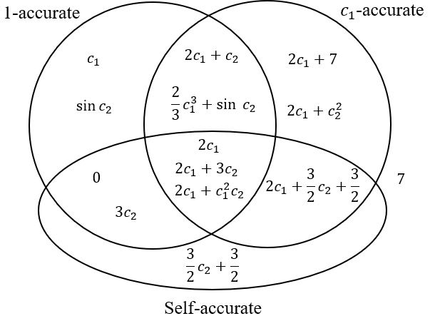
To get some intuition for accuracy, you could verify that the Venn diagram is correct. Another exercise: find another estimator that goes in the center of the Venn diagram. This Wikipedia page may be useful.
(Multi-)accuracy is closely related to linear regression. In particular, the OLS (i.e. linear regression) estimator[15] of \(Y\) in terms of a set of predictors \(S = {X_1, \ldots, X_n}\) is \(S\)-multiaccurate (and is the only \(S\)-multiaccurate estimator that is a linear combination of \(X_1, \ldots, X_n\)). The linear regression estimator is also self-accurate.[16]
We can adapt our definition of accuracy for estimators (in the probability theory sense used above) to heuristic estimators \(\mathbb{G}\). The basic idea is to replace the estimator \(f\) with our heuristic estimator \(\mathbb{G}\), i.e. to substitute \(\mathbb{G}(Y \mid \Pi)\) for \(f(Y)\):
Definition (accuracy of a heuristic estimator.) Let \(\mathcal{Y}, \mathcal{D}\) be as in the previous definition. Let \(\mathbb{G}\) be a heuristic estimator and \(X: \mathcal{Y} \to \mathbb{R}\) be a random variable. A set of heuristic arguments \(\Pi_X\) makes \(\mathbb{G}\) be \(X\)-accurate over \(\mathcal{D}\) if for all \(\Pi \supseteq \Pi_X\), \(\mathbb{G}(Y \mid \Pi)\) is an \(X\)-accurate estimator over \(\mathcal{D}\) – that is,
\[\mathbb{E}_{Y \sim \mathcal{D}}[(Y - \mathbb{G}(Y \mid \Pi))X] = 0.\]
We say that \(\mathbb{G}\) is \(X\)-accurate over \(\mathcal{D}\) if there is a short \(\Pi_X\) that makes \(\mathbb{G}\) be \(X\)-accurate over \(\mathcal{D}\). We say that \(\mathbb{G}\) is \(S\)-multiaccurate over \(\mathcal{D}\) if \(\mathbb{G}\) is \(X\)-accurate over \(\mathcal{D}\) for all\(\) \(X \in S\).
(The paper clarifies some details that have been skipped over in this definition. For example, the paper defines "short" and clarifies some subtleties around the interpretation of \(\mathbb{G}(Y \mid \Pi)\) in the context of the definition.)
(Note also the similarity between this equation and our definitions of iterated estimation and error orthogonality. Indeed, we recover the definition of iterated estimation in the special case of \(X = 1\) – except that the outer \(\mathbb{G}\) is replaced by an expectation over \(\mathcal{D}\). We can similarly recover error orthogonality in the case of \(X = \mathbb{G}(Y \mid \Pi)\) – see the paper for details, including for a definition of self-accuracy for heuristic estimators.)
While iterated estimation and error orthogonality are primarily "soundness" conditions on \(\mathbb{G}\) – that is, they constrain \(\mathbb{G}\) to output internally consistent estimates – accuracy can additionally be used as a "completeness" condition. In particular, if \(\mathbb{G}\) is \(S\)-multiaccurate, this means that:
- \(\mathbb{G}\) can successfully incorporate the predictors in \(S\) into its estimates; and that
- \(\mathbb{G}\) can reasonably merge its estimates based on these predictors (because if \(X_1, X_2 \in S\) then \(\mathbb{G}(Y \mid \Pi_{X_1} \cup \Pi_{X_2})\) needs to be an \(X_1\)-accurate estimator of \(Y\) and also an \(X_2\)-accurate estimator of \(Y\)).
Now, our goal is for \(\mathbb{G}\) to be \(S\)-multiaccurate for a rich class of predictors \(S\). Such a \(\mathbb{G}\) would be powerful while producing reasonable estimates. Unfortunately, as we discuss in the next section, it seems quite difficult to produce such a \(\mathbb{G}\).
Challenges with the objective approach
Given a natural distribution \(\mathcal{D}\) over mathematical expressions and a small, simple, and natural set of predictors \(S\), it is always possible to efficiently produce a self-accurate and \(S\)-multiaccurate estimator?
It may seem like the answer is yes: in particular, we mentioned earlier that the linear regression of \(Y\) onto the predictors in \(S\) is self-accurate and \(S\)-multiaccurate. However, this raises an important question: can we efficiently compute the necessary regression coefficients?
Unfortunately, as we will discuss, the answer to this question is no.
Estimating the product of jointly normal random variables
Here is a quite simple and natural estimation problem: given a \(n \times n\) covariance matrix \(\Sigma\), estimate the expected product of \(n\) random variables with mean \(0\) and covariance matrix \(\Sigma\).
We consider this estimation problem for two reasons. On the one hand, this is one of the simplest estimation problems for which computing (or even approximating) the correct answer is computationally intractable. On the other hand, this problem captures the core difficulty of a natural, more general estimation problem: estimating the average output of an arithmetic circuit (a circuit with addition and multiplication gates). Addition gates are straightforward: \(\mathbb{G}(X + Y \mid \Pi) = \mathbb{G}(X \mid \Pi) + \mathbb{G}(Y \mid \Pi)\), and so the challenge lies in the multiplication gates.
It turns out that the answer to this estimation problem is equal to the sum of all \(n/2\)-fold products of covariances in which each variable is used exactly once. That is, if \(Z_1, \ldots, Z_n\) are jointly normal, zero-mean random variables, then
\[\mathbb{E}[Z_1 \ldots Z_n] = \sum_{p \in \mathcal{P} _ 2(n)} \prod_{(i, j) \in p} \text{Cov}(Z_i, Z_j),\]
where \(\mathcal{P} _ 2(n)\) denotes the set of all pairings of \({1, \ldots, n}\) (for example, one element of \(\mathcal{P} _ 2(6)\) is \({(1, 4), (2, 3), (5, 6)}\)). (This is called the hafnian of the covariance matrix.)
And so our estimation problem amounts to computing a giant sum. This suggests a natural class of predictors: namely, partial sums.
Concretely, let \(Y = Y(\Sigma)\) be the expected product of random variables with mean zero and covariance matrix \(\Sigma\), and let \(\mathcal{D}\) be the distribution over \(Y\) induced by selecting the (off-diagonal) entries of \(\Sigma\) independently from \(\mathcal{N}(0, 1)\).[17] Given a pairing \(p\) of \({1, \ldots, n}\), we define \(X_p := \prod_{(i, j) \in p} \Sigma_{i, j}\), and for a subset \(S \subseteq \mathcal{P} _ 2(n)\), we define \(X_S := \sum_{p \in S} X_p\) (so \(Y = X_{\mathcal{P} _ 2(n)}\)).
Note that \(X_S\) can be efficient to compute even for exponentially large sets of pairings \(S\). For example, let \(S\) be the set of \(3^{n/4}\) pairings that pair 1, 2, 3, 4 amongst themselves (there are three ways to do so); pair 5, 6, 7, 8, amongst themselves; and so on. Then
\[X_S = (\Sigma_{1, 2} \Sigma_{3, 4} + \Sigma_{1, 3} \Sigma_{2, 4} + \Sigma_{1, 4} \Sigma_{2, 3})(\Sigma_{5, 6} \Sigma_{7, 8} + \Sigma_{5, 7} \Sigma_{6, 8} + \Sigma_{5, 8} \Sigma_{6, 7})(\ldots).\]
And so we might wonder: given two efficiently computable partial sums \(X_{S_1}, X_{S_2}\), is it always possible to efficiently combine them into a single estimate of \(Y\) with linear regression? That is, are the requisite regression coefficients efficiently computable?
Alas, the answer is no. We show this by reduction from 3SAT – that is, we show that if you can compute these regression coefficients, then you can solve boolean satisfiability problem, which is NP-complete. If you're interested in the details, check out Section 4.1 of the paper!
(We have not ruled out the possibility that there is a more sophisticated way to accurate merge the estimators \(X_{S_1}\) and \(X_{S_2}\), given that linear regression is intractable. However, we conjecture that no accurate and efficiently computable merge exists. That is, in general, there is no estimator \(f\) of \(Y\) that is both efficiently computable and \({f, X_{S_1}, X_{S_2}}\)-multiaccurate.)
Even though you can't efficiently compute the regression coefficients for merging these arguments exactly, you might wonder whether it's possible to compute them approximately. Concretely, given sets \(S_1, \ldots, S_m\) for which the predictors \(X_{S_i}\) are efficient to compute, is it possible to find a linear combination of the \(X_{S_i}\)'s that is approximately self-accurate and \({X_{S_1}, \ldots, X_{S_m}}\)-multiaccurate? It turns out that, in order to compute the regression coefficients of \(Y\) onto \(X_{S_1}, \ldots, X_{S_m}\), it is sufficient to compute \(|S_i \cap S_j|\) for all \(i, j\). This suggests that you can estimate the regression coefficients by estimating the sizes of these intersections, which you can do e.g. by randomly sampling elements of \(S_i\) and seeing if they belong to \(S_j\).
It turns out that the number of samples you need depends polynomially on the condition number of the correlation matrix of \(X_{S_1}, \ldots, X_{S_m}\). Unfortunately, this conditional number can be exponentially large.[18]
Currently we do not know how to merge these estimates even approximately, although we aren't confident that this cannot be done. At the very least, the most straightforward approaches do not work, which suggests a barrier to creating algorithms that accurately merge even simple estimates for simple and natural estimation problems.
Estimating the permanent of a matrix
We consider another natural estimation problem: given an \(n \times n\) matrix \(A\), estimate its permanent. The permanent of \(A\) is the sum of all products of \(n\) elements of \(A\), one per row and column:
\[\text{perm}(A) = n! \mathbb{E} _ {\sigma \sim S_n} \left[ \prod_{i = 1}^n A_{i, \sigma(i)} \right].\]
While superficially similar to the determinant, the determinant can be computed efficiently, while the permanent cannot even be approximated efficiently.
In the paper, we consider three different estimates of the permanent, all of which are motivated by an argument via presumption of independence. The row sum estimate is given by
\[E_{\text{row}}(A) := n! \prod_{i = 1}^n \mathbb{E} _ {\sigma \sim S_n}[A_{i, \sigma(i)}] = \frac{n!}{n^n} \prod_{i = 1}^n \sum_{j = 1}^n A_{i, j}.\]
The row sum estimate is \(n!\) times the average product obtained by taking one element of each row of \(A\). It is also the average permanent of all matrices obtained from \(A\) by shuffling each row independently. Similarly, the column sum estimate is given by
\[E_{\text{col}}(A) := \frac{n!}{n^n} \prod_{j = 1}^n \sum_{i = 1}^n A_{i, j}.\]
Finally, the matrix sum estimate is \(n!\) times the average product obtained by taking \(n\) random elements of \(A\) (with replacement):
\[E_{\text{ms}}(A) := \frac{n!}{n^{2n}} \left( \sum_{i = 1}^n \sum_{j = 1}^n A_{i, j} \right)^n.\]
If we want to accurately merge these estimates over a distribution of matrices, we can do so with linear regression. However, the resulting estimator can have undesirable properties. For example, the linear regression estimator over the distribution of matrices with each entry selected independently from \(\mathcal{N}(0, 1)\) takes the form \(\alpha(E_\text{row}(A) + E_{\text{col}}(A)) - \beta E_{\text{ms}}(A)\), where \(\beta\) is positive. In particular, this means that even if \(A\) has exclusively non-negative entries, this linear regression estimate for the permanent of \(A\) can be negative.
This by itself is okay: we do not expect estimates to be reasonable by default. What we do expect, however, is that upon noticing that an estimate is unreasonable, we should be able to correct it. That is, we ought to be able to produce an estimator that merges \(\)the row sum, column sum, and matrix sum estimates, and is non-negative on matrices with non-negative entries.
Unfortunately, we are not aware of a natural way to produce such an estimator. Actually, for matrices with non-negative entries, there is a natural estimator that "merges" the row sum, column sum, and matrix sum estimates: namely, \(\frac{E_{\text{row}} E_{\text{col}}}{E_{\text{ms}}}\). (See Section 5.2 of the paper for an explanation of where this estimator comes from and why it is reasonable.) However, this estimator does not satisfy any accuracy properties over any natural distribution of matrices. This makes sense, because this estimator is "multiplicative" in nature, whereas accuracy is an "additive" property.
Our discussion of estimating the permanent thus poses another barrier to using multiaccuracy to formalize the principle of unpredictable errors. Namely, accuracy forces us to reject a seemingly reasonable estimator while forcing us to create seemingly unnatural estimators to satisfy additional properties (like estimating the permanents of matrices with non-negative entries as being non-negative).
Conclusion
The ultimate goal of formalizing properties like the principle of unpredictable errors it to help guide the search for a heuristic estimator. Once you have formal properties, you can pose a formal mathematical question: "Does there exist a polynomial-time algorithm \(\mathbb{G}: {\text{mathematical expressions}} \times {\text{sets of arguments}} \to \mathbb{R}\) that satisfies [formal properties like linearity, unpredictable errors, etc.]?". Once you have such a question, you can use your mathematical toolbox to try to resolve it. By contrast, without such a question, you're forced to answer vague subjective questions like "What would a reasonable heuristic estimator do in this situation?".
Two properties that have stood the test of time are linearity and respect for proofs. Linearity states that for \(a, b \in \mathbb{R}\) and mathematical expressions \(X, Y\), we have that \(\mathbb{G}(aX + bY \mid \Pi) = a \mathbb{G}(X \mid \Pi) + b \mathbb{G}(Y \mid \Pi).\) Respect for proofs states that, given a proof that \(Y \ge 0\), the proof may be turned into a heuristic argument \(\pi\) such that for all \(\Pi\) containing \(\pi\), we have \(\mathbb{G}(Y \mid \Pi) \ge 0\). Unfortunately, these two properties alone are insufficient to pin down the behavior of \(\mathbb{G}\): there are heuristic estimators that satisfy linearity and respect for proofs but behave "unreasonably" (see Chapter 9 here).
It would be really nice if we could formalize the principle of unpredictable errors, because perhaps a satisfying formalization of this principle, together with linearity and respect for proofs, would force \(\mathbb{G}\) to behave reasonably. So far, we have not found a satisfying formalization; finding one might constitute an important step forward in our understanding of heuristic estimation.
This year, though, we have mostly focused on a different approach. Our new approach reframes the heuristic estimation problem as an activation modeling problem: learning a coherent representation of the statistical properties of a neural network's activations (or the values of a circuit's wires) that lets us answer questions about the neural network (or circuit).[19] We haven't written about this perspective in detail yet, because we are still developing it, but see our recent blog post on estimating tail risks in neural networks for an outline of what this approach might look like. We are excited to see where our new perspective takes us!
Cross-postings for comments: Alignment Forum, LessWrong
Our original notation is \(\tilde{\mathbb{E}}(Y, \pi_1, \ldots, \pi_m)\). In our new work, we use the notation \(\mathbb{G}(Y \mid \pi_1, \ldots, \pi_m)\) to emphasize that, while there are similarities between heuristic estimation and expected values, they are importantly different. ↩︎
See here for an earlier blog post that introduced the mechanistic anomaly detection problem. ↩︎
Perhaps instead of no arguments, \(\mathbb{G}\) is given a short argument that points out that there are twenty digits and that its estimate for each digit ought to be (4.5). ↩︎
Here, "short" means "about as large as the model itself." ↩︎
For example, \(L\) could be based on a trained reward predictor, as in RLHF. ↩︎
For example, if \(M\) is a financial assistant that takes actions such as buying stocks and transferring money between bank accounts, then \(M\) might have a low loss on \(\mathcal{D}\) because it makes good financial decisions, but a low loss on \(x^\ast\) because it implements a money laundering scheme that \(L\) fails to notice. ↩︎
One of the most important and difficult questions faced by this approach is how to find such a \(\Pi\). If the space of arguments is parameterized, then we may hope to learn \(\Pi\) via gradient descent in parallel with training \(M\) itself. ↩︎
The idea is that, without any arguments, \(\mathbb{G}\) does not understand anything about the structure of \(M\), and so should estimate \(M\)'s loss as if \(M\) were a randomly initialized neural network. (Such a network would incur high loss.) Heuristic arguments that explain \(M\)'s structure should cause \(\mathbb{G}\)'s estimate of \(M\)'s loss to decrease. ↩︎
For example, in the iterated distillation and amplification process, \(f\) could be a distillation of a trusted model \(s\); however, we may not trust \(f\). ↩︎
Most generally, the law of iterated expectations states that for a probability space \((\Omega, \mathcal{F}, \mathbb{P})\) with \(\sigma\)-algebras \(\mathcal{H}' \subseteq \mathcal{H} \subseteq \mathcal{F}\), for any integrable random variable \(Y\) we have \(\mathbb{E}[\mathbb{E}[Y \mid \mathcal{H}] \mid \mathcal{H}'] = \mathbb{E}[Y \mid \mathcal{H}']\). ↩︎
It may seem like a generalization (consider the case of \(X=1\)), but it is not: deriving iterated estimation from error orthogonality would require assuming additional properties of \(\mathbb{G}\). ↩︎
The projection law states that for a probability space \((\Omega, \mathcal{F}, \mathbb{P})\) with \(\sigma\)-algebras \(\mathcal{H}' \subseteq \mathcal{H} \subseteq \mathcal{F}\), for square-integrable random variables \(X, Y\), we have \(\mathbb{E}[(Y - \mathbb{E}[Y \mid \mathcal{H}]) \cdot \mathbb{E}[X \mid \mathcal{H}] \mid \mathcal{H}'] = 0\).\(\) ↩︎
As an analogy, consider a proof verifier \(V\) that takes as input a mathematical statement \(x\) and a purported proof \(\pi\), and outputs \(1\) (accept) or \(0\) (reject) depending on whether \(\pi\) is a proof of \(x\). Let \(s(x, \pi)\) be the statement "If \(V(x, \pi) = 1\), then \(x\)." For every \((x, \pi)\), there is a proof \(\pi'\) of \(s(x, \pi)\) (specifically: if \(V(x, \pi) = 1\), then \(\pi\) proves \(x\) and thus \(s(x, \pi)\); and if \(V(x, \pi) = 0\), then the computational trace of \(V\) on \((x, \pi)\) shows that \(V(x, \pi) = 0\) and thus proves \(s(x, \pi)\)). However, \(V\) should not treat the input \((s(x, \pi), \pi')\) as a special case; instead, \(V\) should verify that \(\pi'\) proves \(s(x, \pi)\) just as it would verify any other proof. ↩︎
The term "multiaccuracy" originates in the algorithmic fairness literature, where it is used to describe a predictor that appears unbiased to a given set of statistical tests (see e.g. here and here). ↩︎
Without a constant term. If you want a constant term, you can add the predictor \(1\) to \(S\). ↩︎
Here we speak of the exact linear regression estimator of \(Y\) in terms of \(X_1, \ldots, X_n\): in other words, the linear combination of these predictors that is closest to \(Y\) (in terms of expected squared error over \(\mathcal{D}\)). This contrasts with the more typical setting for linear regression, in which coefficients are computed only approximately based on samples. ↩︎
The diagonal entries (which do not matter for the value of \(Y_\Sigma\)) can always be chosen so that \(\Sigma\) is a valid covariance matrix, simply by making those entries be very large. ↩︎
We believe that by using ridge regression instead of linear regression, it is possible to find an approximately \({X_{S_1}, \ldots, X_{S_m}}\)-multiaccurate estimate of \(Y\). However, this estimate is not approximately self-accurate. See Remark 4.14 in the paper for an explanation for why we consider self-accuracy to be important. ↩︎
Very loosely speaking, the correspondence between heuristic estimation and activation modeling is that a particular activation model corresponds to \(\mathbb{G}(\cdot \mid \Pi)\), and so an activation model can take as input a quantity and return an estimate of that quantity. ↩︎